8. Applications of Eigenvalues and Eigenvectors

Why are eigenvalues and eigenvectors important? Let's look at some real life applications of the use of eigenvalues and eigenvectors in science, engineering and computer science.

a. Google's PageRank

Google's extraordinary success as a search engine was due to their clever use of eigenvalues and eigenvectors. From the time it was introduced in 1998, Google's methods for delivering the most relevant result for our search queries has evolved in many ways, and PageRank is not really a factor any more in the way it was at the beginning.

Google's home page in 1998

But for this discussion, let's go back to the original idea of PageRank.

Let's assume the Web contains 6 pages only. The author of Page 1 thinks pages 2, 4, 5, and 6 have good content, and links to them. The author of Page 2 only likes pages 3 and 4 so only links from her page to them. The links between these and the other pages in this simple web are summarised in this diagram.

A simple Internet web containing 6 pages

Google engineers assumed each of these pages is related in some way to the other pages, since there is at least one link to and from each page in the web.

Their task was to find the "most important" page for a particular search query, as indicated by the writers of all 6 pages. For example, if everyone linked to Page 1, and it was the only one that had 5 incoming links, then it would be easy - Page 1 would be returned at the top of the search result.

However, we can see some pages in our web are not regarded as very important. For example, Page 3 has only one incoming link. Should its outgoing link (to Page 5) be worth the same as Page 1's outgoing link to Page 5?

The beauty of PageRank was that it regarded pages with many incoming links (especially from other popular pages) as more important than those from mediocre pages, and it gave more weighting to the outgoing links of important pages.

Google's use of eigenvalues and eigenvectors

For the 6-page web illustrated above, we can form a "link matrix" representing the relative importance of the links in and out of each page.

Considering Page 1, it has 4 outgoing links (to pages 2, 4, 5, and 6). So in the first column of our "links matrix", we place value `1/4` in each of rows 2, 4, 5 and 6, since each link is worth `1/4` of all the outgoing links. The rest of the rows in column 1 have value `0`, since Page 1 doesn't link to any of them.

Meanwhile, Page 2 has only two outgoing links, to pages 3 and 4. So in the second column we place value `1/2` in rows 3 and 4, and `0` in the rest. We continue the same process for the rest of the 6 pages.

Next, to find the eigenvalues.

`| bb(A) -lambda I |=|(-lambda,0,0,0,1/2,0),(1/4,-lambda,0,0,0,0),(0,1/2,-lambda,0,0,0),(1/4,1/2,0,-lambda,1/2,0),(1/4,0,1,1,-lambda,1),(1/4,0,0,0,0,-lambda)|`

`=lambda^6 - (5lambda^4)/8 - (lambda^3)/4 - (lambda^2)/8`

This expression is zero for `lambda = -0.72031,` `-0.13985+-0.39240j,` `0,` `1`. (I expanded the determinant and then solved it for zero using Wolfram|Alpha.)

We can only use non-negative, real values of `lambda` (since they are the only ones that will make sense in this context), so we conclude `lambda=1.` (In fact, for such PageRank problems we always take `lambda=1`.)

We could set up the six equations for this situation, substitute and choose a "convenient" starting value, but for vectors of this size, it's more logical to use a computer algebra system. Using Wolfram|Alpha, we find the corresponding eigenvector is:

As Page 5 has the highest PageRank (of 8 in the above vector), we conclude it is the most "important", and it will appear at the top of the search results.

We often normalize this vector so the sum of its elements is `1.` (We just add up the amounts and divide each amount by that total, in this case `20`.) This is OK because we can choose any "convenient" starting value and we want the relative weights to add to `1.` I've called this normalized vector `bb(P)` for "PageRank".

Search engine reality checks

1. Our example web above has 6 pages, whereas Google (and Bing and other sesarch engines) needs to cope with billions of pages. This requires a lot of computing power, and clever mathematics to optimize processes.
2. PageRank was only one of many ranking factors employed by Google from the beginning. They also looked at key words in the search query and compared that to the number of times those search words appeared on a page, and where they appeared (if they were in headings or page descriptions they were "worth more" than if the words were lower down the page). All of these factors were fairly easy to "game" once they were known about, so Google became more secretive about what it uses to rank pages for any particular search term.
3. Google currenly use over 200 different signals when analyzing Web pages, including page speed, whether local or not, mobile friendliness, amount of text, authority of the overall site, freshness of the content, and so on. They constantly revise those signals to beat "black hat" operators (who try to game the system to get on top) and to try to ensure the best quality and most authoritative pages are presented at the top.

References and further reading

1. How Google Finds Your Needle in the Web's Haystack (a good explanation of the basics of PageRank and consideration of cases that don't quite fit the model)
2. The Anatomy of a Large-Scale Hypertextual Web Search Engine (the original Stanford research paper by Sergey Brin and Lawrence Page presenting the concepts behind Google search, using eigenvalues and eigenvectors)
3. The $25,000,000,000 Eigenvector The Linear Algebra Behind Google (PDF, containing further explanation)

b. Electronics: RLC circuits

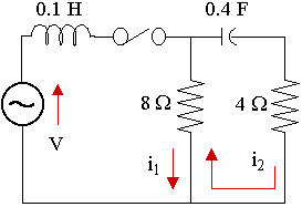
An electical circuit consists of 2 loops, one with a 0.1 H inductor and the second with a 0.4 F capacitor and a 4 Ω resistor, and sharing an 8 Ω resistor, as shown in the diagram. The power supply is 12 V. (We'll learn how to solve such circuits using systems of differential equations in a later chapter, beginning at Series RLC Circuit.)

Let's see how to solve such a circuit (that means finding the currents in the two loops) using matrices and their eigenvectors and eigenvalues. We are making use of Kirchhoff's voltage law and the definitions regarding voltage and current in the differential equations chapter linked to above.

NOTE: There is no attempt here to give full explanations of where things are coming from. It's just to illustrate the way such circuits can be solved using eigenvalues and eigenvectors.

For the left loop: `0.1(di_1)/(dt) + 8(i_1 - i_2) = 12`

Muliplying by 10 and rearranging gives: `(di_1)/(dt) = - 80i_1 + 80i_2 +120` . (1)

For the right loop: `4i_2 + 2.5 int i_2 dt + 8(i_2 - i_1) = 12`

Differentiating gives: `4(di_2)/(dt) + 2.5i_2 + 8((di_2)/(dt) - (di_1)/(dt)) = 12`

Rearranging gives: `12(di_2)/(dt) = 8(di_1)/(dt) - 2.5i_2 + 12`

Substituting (1) gives: `12(di_2)/(dt)` ` = 8(- 80i_1 + 80i_2 +120) - 2.5i_2 + 12` ` = - 640i_1 + 637.5i_2 + 972`

Dividing through by 12 and rearranging gives: `(di_2)/(dt) = - 53.333i_1 + 53.125i_2 + 81` . (2)

We can write (1) and (2) in matrix form as:

`(dbb(K))/(dt) = bb(AK) + bb(v)`, where `bb(K)=[(i_1),(i_2)],` `bb(A) = [(-80, 80),(-53.333, 53.125)],` `bb(v)=[(120),(81)]`

The characteristic equation for matrix A is `lambda^2 + 26.875lambda + 16.64 = 0` which yields the eigenvalue-eigenvector pairs `lambda_1=-26.2409,` `bb(v)_1 = [(1.4881),(1)]` and `lambda_2=-0.6341,` `bb(v)_2 = [(1.008),(1)].`

The eigenvectors give us a general solution for the system:

c. Repeated applications of a matrix: Markov processes

Scenario: A market research company has observed the rise and fall of many technology companies, and has predicted the future market share proportion of three companies A, B and C to be determined by a transition matrix P, at the end of each monthly interval:

The first row of matrix P represents the share of Company A that will pass to Company A, Company B and Company C respectively. The second row represents the share of Company B that will pass to Company A, Company B and Company C respectively, while the third row represents the share of Company C that will pass to Company A, Company B and Company C respectively. Notice each row adds to 1.

The initial market share of the three companies is represented by the vector `bb(s_0)=[(30),(15),(55)]`, that is, Company A has 30% share, Company B, 15% share and Company C, 55% share.

We can calculate the predicted market share after 1 month, s₁, by multiplying P and the current share matrix:

Next, we can calculate the predicted market share after the second month, s₂, by squaring the transition matrix (which means applying it twice) and multiplying it by s₀:

`bb(s)_2` `=bb(P)^2bb(s_0)` `=[(0.663,0.18,0.157),(0.0565,0.9065,0.037),(0.3115,0.105,0.5835)][(30),(15),(55)]` `= [(37.87),(24.7725),(37.3575)]`

Continuing in this fashion, we see that after a period of time, the market share of the three companies settles down to around 23.8%, 61.6% and 14.5%. Here's a table with selected values.

This type of process involving repeated multiplication of a matrix is called a Markov Process, after the 19th century Russian mathematician Andrey Markov.

Here's the graph of the change in proportions over a period of 40 months.